Poisson equation in 1D
Problem setup
We will learn the solution operator
for the one-dimensional Poisson problem
with zero Dirichlet boundary conditions \(u(0) = u(1) = 0\).
The source term \(f\) is supposed to be an arbitrary continuous function.
Implementation
The solution operator can be learned by training a physics-informed DeepONet.
First, we define the PDE with boundary conditions and the domain:
def equation(x, y, f):
    dy_xx = dde.grad.hessian(y, x)
    return -dy_xx - f

geom = dde.geometry.Interval(0, 1)

def u_boundary(_):
    return 0

def boundary(_, on_boundary):
    return on_boundary

bc = dde.icbc.DirichletBC(geom, u_boundary, boundary)

pde = dde.data.PDE(geom, equation, bc, num_domain=100, num_boundary=2)
Next, we specify the function space for \(f\) and the corresponding evaluation points.
For this example, we use the dde.data.PowerSeries to get the function space
of polynomials of degree three.
Together with the PDE, the function space is used to define a
PDEOperator dde.data.PDEOperatorCartesianProd that incorporates the PDE into
the loss function.
degree = 3
space = dde.data.PowerSeries(N=degree + 1)

num_eval_points = 10
evaluation_points = geom.uniform_points(num_eval_points, boundary=True)

pde_op = dde.data.PDEOperatorCartesianProd(
    pde,
    space,
    evaluation_points,
    num_function=100,
)
The DeepONet can be defined using dde.nn.DeepONetCartesianProd.
The branch net is chosen as a fully connected neural network of size [m, 32, p] where p=32
and the trunk net is a fully connected neural network of size [dim_x, 32, p].
dim_x = 1
p = 32
net = dde.nn.DeepONetCartesianProd(
    [num_eval_points, 32, p],
    [dim_x, 32, p],
    activation="tanh",
    kernel_initializer="Glorot normal",
)
We define the Model and train it with L-BFGS:
model = dde.Model(pde_op, net)
dde.optimizers.set_LBFGS_options(maxiter=1000)
model.compile("L-BFGS")
model.train()
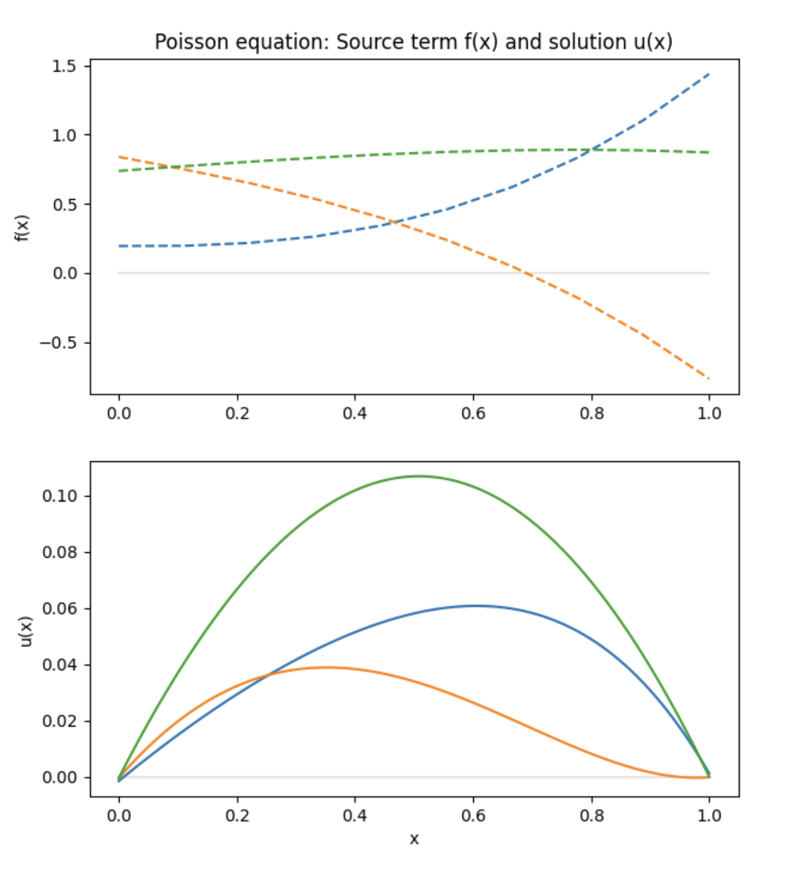
Finally, the trained model can be used to predict the solution of the Poisson equation. We sample the solution for three random representations of \(f\).
n = 3
features = space.random(n)
fx = space.eval_batch(features, evaluation_points)

x = geom.uniform_points(100, boundary=True)
y = model.predict((fx, x))
Complete code
"""Backend supported: tensorflow.compat.v1, tensorflow, pytorch, paddle"""
import deepxde as dde
import matplotlib.pyplot as plt
import numpy as np


# Poisson equation: -u_xx = f
def equation(x, y, f):
    dy_xx = dde.grad.hessian(y, x)
    return -dy_xx - f


# Domain is interval [0, 1]
geom = dde.geometry.Interval(0, 1)


# Zero Dirichlet BC
def u_boundary(_):
    return 0


def boundary(_, on_boundary):
    return on_boundary


bc = dde.icbc.DirichletBC(geom, u_boundary, boundary)

# Define PDE
pde = dde.data.PDE(geom, equation, bc, num_domain=100, num_boundary=2)

# Function space for f(x) are polynomials
degree = 3
space = dde.data.PowerSeries(N=degree + 1)

# Choose evaluation points
num_eval_points = 10
evaluation_points = geom.uniform_points(num_eval_points, boundary=True)

# Define PDE operator
pde_op = dde.data.PDEOperatorCartesianProd(
    pde,
    space,
    evaluation_points,
    num_function=100,
)

# Setup DeepONet
dim_x = 1
p = 32
net = dde.nn.DeepONetCartesianProd(
    [num_eval_points, 32, p],
    [dim_x, 32, p],
    activation="tanh",
    kernel_initializer="Glorot normal",
)

# Define and train model
model = dde.Model(pde_op, net)
dde.optimizers.set_LBFGS_options(maxiter=1000)
model.compile("L-BFGS")
model.train()

# Plot realisations of f(x)
n = 3
features = space.random(n)
fx = space.eval_batch(features, evaluation_points)

x = geom.uniform_points(100, boundary=True)
y = model.predict((fx, x))

# Setup figure
fig = plt.figure(figsize=(7, 8))
plt.subplot(2, 1, 1)
plt.title("Poisson equation: Source term f(x) and solution u(x)")
plt.ylabel("f(x)")
z = np.zeros_like(x)
plt.plot(x, z, "k-", alpha=0.1)

# Plot source term f(x)
for i in range(n):
    plt.plot(evaluation_points, fx[i], "--")

# Plot solution u(x)
plt.subplot(2, 1, 2)
plt.ylabel("u(x)")
plt.plot(x, z, "k-", alpha=0.1)
for i in range(n):
    plt.plot(x, y[i], "-")
plt.xlabel("x")

plt.show()