PI-DeepONets with Zero Coordinate Shift (ZCS)

Zero Coordinate Shift (ZCS) is a low-level technique for maximizing memory and time efficiency of physics-informed DeepONets (Leng et al., 2023). In this tutorial, we will explain how to activate ZCS in an existing DeepXDE script. Usually, ZCS can reduce GPU memory consumption and wall time for training by an order of magnitude.

Prerequisite

Your current script can be easily equipped with ZCS if you are using

TensorFlow 2.x, PyTorch or Paddle as the backend (use PyTorch for best performance),
dde.data.PDEOperatorCartesianProd as the data class, and
dde.nn.DeepONetCartesianProd as the network class.

Usage

Switching to ZCS requires two steps.

Step 1: Replacing the classes in the following table

FROM	TO
`deepxde.data.PDEOperatorCartesianProd`	`deepxde.zcs.PDEOperatorCartesianProd`
`deepxde.Model`	`deepxde.zcs.Model`

Step 2: Changing the PDE equation(s) to ZCS format

In DeepXDE, the user function for the PDE equation(s) is declared as

def pde(x, u, v):
    # ...

To use ZCS, we first create a deepxde.zcs.LazyGrad object, passing x and u as the arguments. The derivatives of u w.r.t. x at any higher orders can then be computed by LazyGrad.compute(orders). For example, the Laplace equation (\(u_{xx}+u_{yy}=0\)) can be coded as

def pde(x, u, v):
    grad_u = dde.zcs.LazyGrad(x, u)
    du_xx = grad_u.compute((2, 0))
    du_yy = grad_u.compute((0, 2))
    return du_xx + du_yy

Note: deepxde.zcs.LazyGrad is smart enough to avoid re-calculating any lower-order derivatives if a higher-order one has been calculated based on them. For example, in the above function, if you add du_x = grad_u.compute((1, 0)) after du_xx = grad_u.compute((2, 0)), du_x will be returned instantly from a cache inside grad_u without extra computation.

These are all you need!

Example 1: diffusion reaction

In this example, we activate ZCS in the demo of diffusion reaction equation. The PDE is \(u_{t} - D u_{xx} + k u^2 -v=0\), which is implemented in the original script as

def pde(x, u, v):
    D = 0.01
    k = 0.01
    du_t = dde.grad.jacobian(u, x, j=1)
    du_xx = dde.grad.hessian(u, x, j=0)
    return du_t - D * du_xx + k * u ** 2 - v

In the ZCS script, we change the PDE to (along with replacing the classes in Step 1)

def pde(x, u, v):
    D = 0.01
    k = 0.01
    grad_u = dde.zcs.LazyGrad(x, u)
    du_t = grad_u.compute((0, 1))
    du_xx = grad_u.compute((2, 0))
    return du_t - D * du_xx + k * u ** 2 - v

The GPU memory and wall time we measured on a Nvidia V100 (with CUDA 12.2) are reported below. For these measurements, we have increased the number of points in the domain from 200 to 4000, as 200 is likely to be insufficient for real applications. Time is measured for 1000 iterations.

BACKEND	METHOD	GPU / MB	TIME / s
PyTorch	Aligned	5779	186
	Unaligned	5873	117
	ZCS	655	11
TensorFlow	Aligned	9205	73 (with jit)
	Unaligned	11694	70 (with jit)
	ZCS	591	35 (no jit^†)
Paddle	Aligned	5805	197
	Unaligned	6923	385
	ZCS	1353	15

^†ZCS with Jit is on our TODO list.

Example 2: Stokes flow

The Problem

In this example, we use a PI-DeepONet to approach the system of Stokes for fluids. The domain is a 2D square full of liquid, with its lid moving horizontally at a given variable speed. The full equations and boundary conditions are

\[\begin{split}\begin{aligned} \mu\left(\frac{\partial^2 u}{\partial x^2} + \frac{\partial^2 u}{\partial y^2}\right) - \frac{\partial p}{\partial x}=0, \quad & x\in (0,1), y\in(0, 1);\\ \mu\left(\frac{\partial^2 v}{\partial x^2} + \frac{\partial^2 v}{\partial y^2}\right) - \frac{\partial p}{\partial y}=0, \quad & x\in (0,1), y\in(0, 1);\\ \frac{\partial u}{\partial x} + \frac{\partial v}{\partial y}=0, \quad & x\in (0,1), y\in(0, 1);\\ u(x,1)=u_1(x), v(x,1)=0, \quad & x\in(0, 1);\\ u(x,0)=v(x,0)=p(x,0)=0, \quad & x\in(0, 1);\\ u(0,y)=v(0,y)=0, \quad & y\in(0, 1);\\ u(1,y)=v(1,y)=0, \quad & y\in(0, 1). \end{aligned}\end{split}\]

We attempt to learn an operator mapping from \(u_1(x)\) to \(\{u, v, p\}(x, y)\), with \(u_1(x)\) sampled from a Gaussian process. The true solution for validation is computed using FreeFEM++ following this tutorial.

PDE implementation

Without ZCS, the script with aligned points implements the PDE as

def pde(xy, uvp, aux):
    mu = 0.01
    # first order
    du_x = dde.grad.jacobian(uvp, xy, i=0, j=0)
    dv_y = dde.grad.jacobian(uvp, xy, i=1, j=1)
    dp_x = dde.grad.jacobian(uvp, xy, i=2, j=0)
    dp_y = dde.grad.jacobian(uvp, xy, i=2, j=1)
    # second order
    du_xx = dde.grad.hessian(uvp, xy, component=0, i=0, j=0)
    du_yy = dde.grad.hessian(uvp, xy, component=0, i=1, j=1)
    dv_xx = dde.grad.hessian(uvp, xy, component=1, i=0, j=0)
    dv_yy = dde.grad.hessian(uvp, xy, component=1, i=1, j=1)
    motion_x = mu * (du_xx + du_yy) - dp_x
    motion_y = mu * (dv_xx + dv_yy) - dp_y
    mass = du_x + dv_y
    return motion_x, motion_y, mass

Accordingly, the script with ZCS implements the PDE as

def pde(xy, uvp, aux):
    mu = 0.01
    u, v, p = uvp[..., 0:1], uvp[..., 1:2], uvp[..., 2:3]
    grad_u = dde.zcs.LazyGrad(xy, u)
    grad_v = dde.zcs.LazyGrad(xy, v)
    grad_p = dde.zcs.LazyGrad(xy, p)
    # first order
    du_x = grad_u.compute((1, 0))
    dv_y = grad_v.compute((0, 1))
    dp_x = grad_p.compute((1, 0))
    dp_y = grad_p.compute((0, 1))
    # second order
    du_xx = grad_u.compute((2, 0))
    du_yy = grad_u.compute((0, 2))
    dv_xx = grad_v.compute((2, 0))
    dv_yy = grad_v.compute((0, 2))
    motion_x = mu * (du_xx + du_yy) - dp_x
    motion_y = mu * (dv_xx + dv_yy) - dp_y
    mass = du_x + dv_y
    return motion_x, motion_y, mass

Both of them should be self-explanatory.

Results

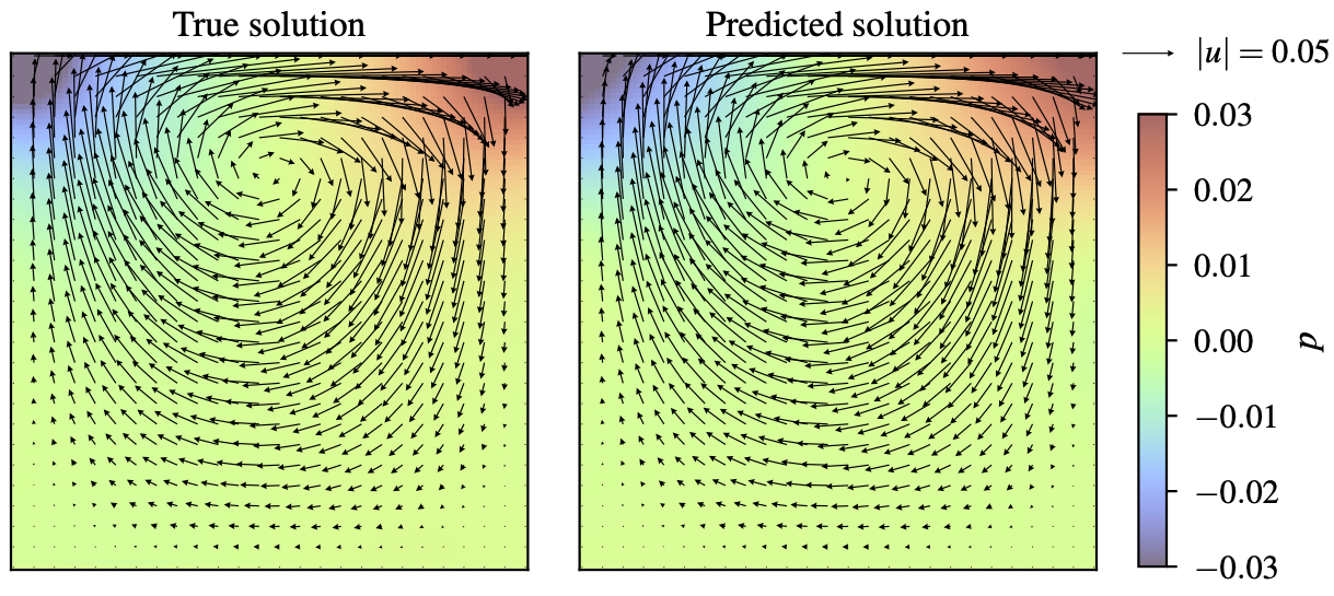
After 50,000 iterations of training, the relative errors for both velocity and pressure should converge to around 10%. The following figure shows the true and the predicted solutions for \(u_1(x)=x(1-x)\). Note that ZCS does not affect the accuracy of the resultant model – it just gears up the training while saving GPU memory. You may want to decrease the number of iterations for a quicker run.

The memory and time measurements on a Nvidia A100 (80 GB, CUDA 12.2) are given below. Note that the wall time is measured for 100 iterations.

BACKEND	METHOD	GPU / MB	TIME / s
PyTorch	Aligned	70630	431
	ZCS	4067	17
TensorFlow	Aligned	Failed^†	Failed^†
	ZCS	8632	81

^†Aligned failed with TensorFlow (v2.15.0) because graphing by @tf.function (either with jit_compile on or off) got stuck on both the two machines we tested on. If you manage to run it successfully, please report the results in an issue.